Getting started
psipy is a package for loading and visualising the output of PSI’s MAS model runs. This page provides some narrative documentation that should get you up and running with obtaining, loading, and visualising some model results.
Getting data
The PSI MHDWeb pages give access to MAS model runs. The runs are indexed by Carrington rotation, and for each Carrington rotation there are generally a number of different runs, varying in the type model run and/or the boundary conditions.
To load data with psipy you need to manually download the files you are interested in to a directory on your computer.
Loading data
psipy stores the output variables from a single MAS run in the
MASOutput object. To create one of these, specify the directory
which has all of the outputs .hdf files you want to load:
from psipy.model import MASOutput

directory = '/path/to/files'
mas_output = MASOutput(directory)
To see which variables have been loaded, we can look at the .variables
attribute:
print(mas_output.variables)
This will print a list of the variables that have been loaded. Each individual variable can then be accessed with square brackets, for example to get the radial magnetic field component:
br = mas_output['br']
This will return a Variable object, which stores the underlying data as a
xarray.DataArray under the Variable.data property.
Data coordinates
The data stored in Variable.data contains the values of the data as a normal
array, and in addition stores the coordinates of each data point.
MAS model outputs are defined on a 3D grid of points on a spherical grid. The
coordinate names are 'r', 'theta', 'phi'. The coordinate values along each
dimension can be accessed using the r_coords, theta_coords, phi_coords
properties, e.g.:
rvals = br.r_coords
Plotting data
Variable objects have methods to plot 2D slices of the data. These
methods are:
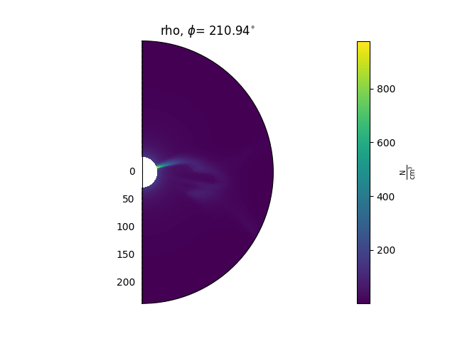
A typical use looks like this:
ax = plt.subplot(1, 1, 1, projection='polar')
model['rho'].plot_phi_cut(index, ax=ax, ...)
and produces an output like this:
For more examples of how to use these methods, see the Examples gallery.
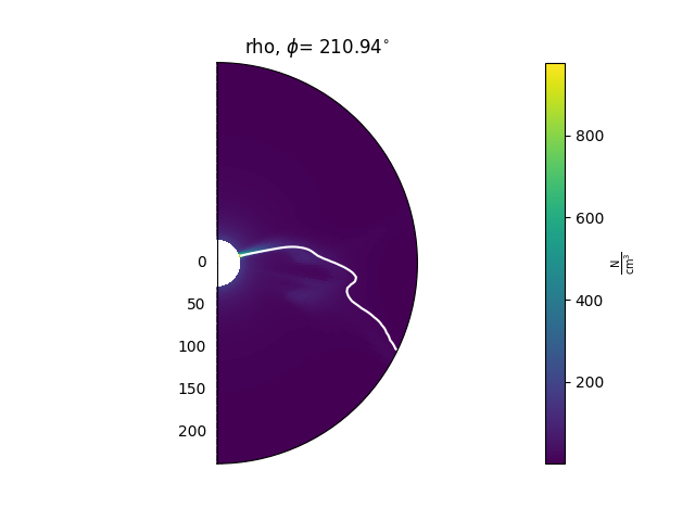
There are also methods that can be used to plot contours of the data on top of these 2D slices. As an example, this can be helpful for plotting the heliospheric current sheet, by contouring \(B_{r} = 0\). These methods are
A typical use looks like this:
ax = plt.subplot(1, 1, 1, projection='polar')
model['rho'].plot_phi_cut(index, ax=ax, ...)
model['br'].contour_phi_cut(index, levels=[0], ax=ax, ...)
and produces outputs like this:
For more examples of how to use these methods, see the Examples gallery.
Normalising data before plotting
Sometimes it is helpful to multiply data by an expected radial falloff, e.g.
multiplying the density by \(r^{2}\). This can be done using the
Variable.radial_normalized method, e.g.:
rho = mas_output['rho']
rho_r_squared = rho.radial_normalized(2)
rho_r_squared.plot_phi_cut(...)
Sampling data
Variable objects have a Variable.sample_at_coords method, to take a sample of
the 3D data cube along a 1D trajectory. This is helpful for flying a ‘virtual
spacecraft’ through the model, in order to compare model results with in-situ
measurements.
sample_at_coords requires arrays of longitude, latitude, and radial distance.
Given these coordinates, it uses linear interpolation to extract the values
of the variable at each of the coordinate points.
For an example of how all this works, see Comparing in-situ data to model output.