Sampling data from a 3D model

In this example we’ll see how to sample a 3D model output at arbitrary points within the model domain.

First, load the required modules.

from psipy.model import MASOutput
from psipy.data import sample_data

import astropy.constants as const
import astropy.units as u

import matplotlib.pyplot as plt
import numpy as np

Load a set of MAS output files, and get the number density variable from the model run.

mas_path = sample_data.mas_helio()
model = MASOutput(mas_path)
rho = model['rho']

Out:

Files Downloaded:   0%|          | 0/3 [00:00<?, ?file/s]


vr002.hdf:   0%|          | 0.00/7.96M [00:00<?, ?B/s]



br002.hdf:   0%|          | 0.00/7.94M [00:00<?, ?B/s]

rho002.hdf:   0%|          | 0.00/8.02M [00:00<?, ?B/s]


vr002.hdf:   0%|          | 2.00/7.96M [00:00<142:42:05, 15.5B/s]

rho002.hdf:   0%|          | 100/8.02M [00:00<2:53:33, 770B/s]



br002.hdf:   0%|          | 100/7.94M [00:00<2:55:46, 753B/s]


vr002.hdf:   0%|          | 31.7k/7.96M [00:00<00:52, 151kB/s]

rho002.hdf:   0%|          | 9.88k/8.02M [00:00<02:51, 46.6kB/s]



br002.hdf:   0%|          | 10.1k/7.94M [00:00<02:48, 47.0kB/s]

rho002.hdf:   1%|          | 53.3k/8.02M [00:00<00:44, 179kB/s]


vr002.hdf:   2%|1         | 159k/7.96M [00:00<00:14, 525kB/s]



br002.hdf:   1%|          | 53.5k/7.94M [00:00<00:44, 176kB/s]

rho002.hdf:   2%|2         | 175k/8.02M [00:00<00:15, 494kB/s]


vr002.hdf:   6%|5         | 475k/7.96M [00:00<00:05, 1.30MB/s]



br002.hdf:   2%|1         | 149k/7.94M [00:00<00:19, 390kB/s]

rho002.hdf:   6%|6         | 499k/8.02M [00:00<00:05, 1.35MB/s]


vr002.hdf:  12%|#2        | 986k/7.96M [00:00<00:02, 2.47MB/s]



br002.hdf:   6%|5         | 447k/7.94M [00:00<00:06, 1.12MB/s]

rho002.hdf:  10%|9         | 796k/8.02M [00:00<00:03, 1.85MB/s]


vr002.hdf:  19%|#9        | 1.53M/7.96M [00:00<00:01, 3.25MB/s]



br002.hdf:   7%|7         | 568k/7.94M [00:00<00:06, 1.09MB/s]

rho002.hdf:  15%|#4        | 1.18M/8.02M [00:00<00:02, 2.46MB/s]


vr002.hdf:  28%|##7       | 2.19M/7.96M [00:00<00:01, 4.25MB/s]



br002.hdf:  10%|9         | 769k/7.94M [00:00<00:05, 1.29MB/s]

rho002.hdf:  19%|#8        | 1.50M/8.02M [00:00<00:02, 2.66MB/s]


vr002.hdf:  39%|###8      | 3.07M/7.96M [00:00<00:00, 5.26MB/s]



br002.hdf:  14%|#4        | 1.15M/7.94M [00:00<00:03, 1.94MB/s]


vr002.hdf:  48%|####7     | 3.78M/7.96M [00:01<00:00, 5.79MB/s]



br002.hdf:  17%|#7        | 1.38M/7.94M [00:01<00:03, 2.04MB/s]



br002.hdf:  23%|##3       | 1.86M/7.94M [00:01<00:02, 2.84MB/s]



br002.hdf:  33%|###3      | 2.64M/7.94M [00:01<00:01, 4.26MB/s]



br002.hdf:  39%|###8      | 3.08M/7.94M [00:01<00:01, 3.51MB/s]


vr002.hdf:  55%|#####4    | 4.37M/7.96M [00:01<00:01, 2.69MB/s]


vr002.hdf:  61%|######    | 4.82M/7.96M [00:01<00:01, 2.64MB/s]



br002.hdf:  44%|####3     | 3.46M/7.94M [00:01<00:02, 2.02MB/s]


vr002.hdf:  65%|######5   | 5.20M/7.96M [00:01<00:01, 2.37MB/s]



br002.hdf:  47%|####7     | 3.76M/7.94M [00:01<00:01, 2.11MB/s]


vr002.hdf:  69%|######9   | 5.52M/7.96M [00:02<00:01, 2.41MB/s]



br002.hdf:  57%|#####6    | 4.49M/7.94M [00:02<00:01, 3.10MB/s]


vr002.hdf:  80%|########  | 6.37M/7.96M [00:02<00:00, 1.92MB/s]



br002.hdf:  62%|######1   | 4.91M/7.94M [00:02<00:02, 1.35MB/s]

rho002.hdf:  22%|##2       | 1.77M/8.02M [00:02<00:15, 394kB/s]


vr002.hdf:  83%|########3 | 6.62M/7.96M [00:02<00:00, 1.49MB/s]



br002.hdf:  66%|######5   | 5.21M/7.94M [00:03<00:01, 1.46MB/s]

rho002.hdf:  25%|##4       | 1.97M/8.02M [00:03<00:12, 471kB/s]


vr002.hdf:  87%|########7 | 6.95M/7.96M [00:03<00:00, 1.68MB/s]



br002.hdf:  70%|######9   | 5.53M/7.94M [00:03<00:01, 1.64MB/s]


vr002.hdf:  93%|#########3| 7.42M/7.96M [00:03<00:00, 2.11MB/s]



br002.hdf:  76%|#######5  | 6.02M/7.94M [00:03<00:00, 2.14MB/s]

rho002.hdf:  29%|##9       | 2.34M/8.02M [00:03<00:08, 678kB/s]


vr002.hdf: 100%|#########9| 7.94M/7.96M [00:03<00:00, 2.63MB/s]



Files Downloaded:  33%|###3      | 1/3 [00:03<00:06,  3.48s/file]



br002.hdf:  82%|########1 | 6.47M/7.94M [00:03<00:00, 2.56MB/s]

rho002.hdf:  36%|###5      | 2.85M/8.02M [00:03<00:04, 1.08MB/s]



br002.hdf:  94%|#########4| 7.50M/7.94M [00:03<00:00, 4.07MB/s]




Files Downloaded:  67%|######6   | 2/3 [00:03<00:01,  1.51s/file]

rho002.hdf:  40%|####      | 3.22M/8.02M [00:03<00:03, 1.31MB/s]

rho002.hdf:  43%|####3     | 3.48M/8.02M [00:03<00:03, 1.24MB/s]

rho002.hdf:  49%|####8     | 3.90M/8.02M [00:03<00:02, 1.61MB/s]

rho002.hdf:  59%|#####8    | 4.71M/8.02M [00:03<00:01, 2.68MB/s]

rho002.hdf:  64%|######4   | 5.14M/8.02M [00:04<00:01, 2.55MB/s]

rho002.hdf:  70%|#######   | 5.61M/8.02M [00:04<00:00, 2.87MB/s]

rho002.hdf:  83%|########2 | 6.62M/8.02M [00:04<00:00, 4.35MB/s]

rho002.hdf:  99%|#########8| 7.93M/8.02M [00:04<00:00, 6.35MB/s]


Files Downloaded: 100%|##########| 3/3 [00:04<00:00,  1.29s/file]
Files Downloaded: 100%|##########| 3/3 [00:04<00:00,  1.55s/file]

Choose a set of 1D points to interpolate the model output at.

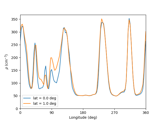
Here we keep a constant radius, and a set of longitudes that go all the way from 0 to 360 degrees. Then we choose two different, but close latitude values, and plot the results.

As expected, the values at 0 and 360 degrees are the same, and the profiles are similar, but different, due to the small difference in latitude.

fig, ax = plt.subplots()

npoints = 1000
r = 50 * np.ones(npoints) * const.R_sun
lon = np.linspace(0, 360, npoints) * u.deg

for latitude in [0, 1] * u.deg:
    lat = latitude * np.ones(npoints)
    samples = rho.sample_at_coords(lon, lat, r)

    ax.plot(lon, samples, label='lat = ' + str(latitude))

ax.legend()
ax.set_xlim(0, 360)
ax.set_ylim(bottom=0)
ax.set_xlabel('Longitude (deg)')
ax.set_ylabel(r'$\rho$ (cm$^{-3}$)')
ax.set_xticks([0, 90, 180, 270, 360])
plt.show()