Sampling data across timesteps

In this example we’ll see how to sample a 3D model across multiple timesteps.

First, load the required modules.

import astropy.units as u
import matplotlib.pyplot as plt
import numpy as np

from psipy.data import sample_data
from psipy.model import MASOutput

Load a set of MAS output files, and get the radial velocity variable from the model run. Note that there are multiple timesteps in the Variable object.

mas_path = sample_data.mas_helio_timesteps()
model = MASOutput(mas_path)
vr = model["vr"]
print(f"Number of timesteps: {vr.n_timesteps}")

  0%|                                              | 0.00/7.96M [00:00<?, ?B/s]
  1%|▍                                     | 98.3k/7.96M [00:00<00:10, 720kB/s]
  6%|██                                    | 442k/7.96M [00:00<00:04, 1.75MB/s]
 15%|█████▍                               | 1.16M/7.96M [00:00<00:02, 3.32MB/s]
 24%|█████████                            | 1.95M/7.96M [00:00<00:01, 4.25MB/s]
 35%|█████████████                        | 2.82M/7.96M [00:00<00:01, 5.08MB/s]
 46%|████████████████▉                    | 3.64M/7.96M [00:00<00:00, 5.03MB/s]
 58%|█████████████████████▍               | 4.60M/7.96M [00:00<00:00, 5.86MB/s]
 67%|████████████████████████▊            | 5.34M/7.96M [00:01<00:00, 5.69MB/s]
 77%|████████████████████████████▎        | 6.09M/7.96M [00:01<00:00, 5.61MB/s]
 86%|███████████████████████████████▊     | 6.85M/7.96M [00:01<00:00, 5.62MB/s]
 94%|██████████████████████████████████▉  | 7.50M/7.96M [00:01<00:00, 5.82MB/s]
  0%|                                              | 0.00/7.96M [00:00<?, ?B/s]
100%|█████████████████████████████████████| 7.96M/7.96M [00:00<00:00, 16.1GB/s]

  0%|                                              | 0.00/7.96M [00:00<?, ?B/s]
  1%|▍                                     | 98.3k/7.96M [00:00<00:10, 715kB/s]
  5%|█▊                                    | 377k/7.96M [00:00<00:05, 1.48MB/s]
 14%|█████▏                               | 1.11M/7.96M [00:00<00:02, 3.23MB/s]
 24%|████████▉                            | 1.93M/7.96M [00:00<00:01, 4.29MB/s]
 35%|█████████████                        | 2.82M/7.96M [00:00<00:01, 5.05MB/s]
 48%|█████████████████▌                   | 3.78M/7.96M [00:00<00:00, 5.65MB/s]
 61%|██████████████████████▌              | 4.85M/7.96M [00:00<00:00, 6.41MB/s]
 73%|██████████████████████████▉          | 5.80M/7.96M [00:01<00:00, 7.19MB/s]
 84%|███████████████████████████████      | 6.67M/7.96M [00:01<00:00, 7.35MB/s]
 97%|███████████████████████████████████▉ | 7.73M/7.96M [00:01<00:00, 8.21MB/s]
  0%|                                              | 0.00/7.96M [00:00<?, ?B/s]
100%|█████████████████████████████████████| 7.96M/7.96M [00:00<00:00, 16.5GB/s]
Number of timesteps: 2

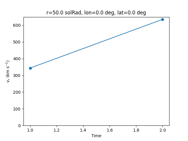
To sample across times, we’ll keep a constant spatial coordinate (r, lat, lon), but sample at each of the time coordinates. This isn’t that exciting because there’s only two timesteps, but illustrates how it works!

fig, ax = plt.subplots()

t = vr.time_coords
r = 50 * u.R_sun * np.ones(len(t))
lon = 0 * u.deg * np.ones(len(t))
lat = 0 * u.deg * np.ones(len(t))

samples = vr.sample_at_coords(lon, lat, r, t)

ax.plot(t, samples, marker="o")

ax.set_ylim(bottom=0)
ax.set_xlabel("Time")
ax.set_ylabel(r"$v_{r}$ (km s$^{-1}$)")
ax.set_title(f"r={r[0]}, lon={lon[0]}, lat={lat[0]}")
plt.show()