Note
Click here to download the full example code
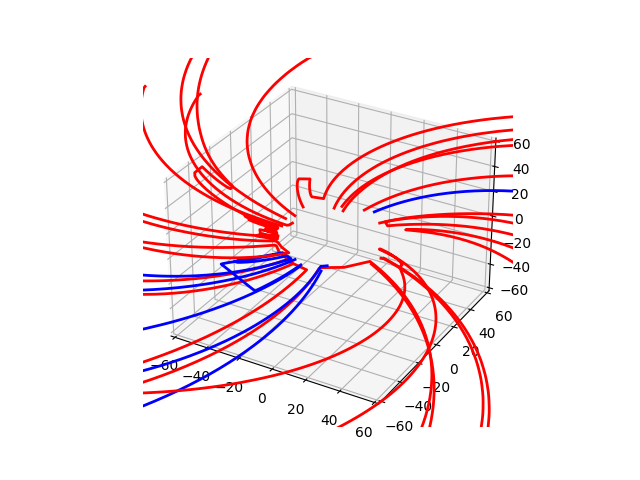
Field lines with Matplotlib
Visualising traced field lines with Matplotlib.
First, load the required modules.
import astropy.units as u
import matplotlib.pyplot as plt
import numpy as np

from psipy.data import sample_data
from psipy.model import MASOutput
from psipy.tracing import FortranTracer
Load a set of MAS output files.
To trace field lines, start by creating a tracer. Then we create a set of seed points at which the field lines are drawn from.
tracer = FortranTracer()

nseeds = 5
# Radius
r = np.ones(nseeds**2) * 40 * u.R_sun
# Some points near the equatorial plane
lat = np.linspace(-10, 10, nseeds**2, endpoint=False) * u.deg
# Choose random longitudes
lon = np.random.rand(nseeds**2) * 360 * u.deg

# Do the tracing!
flines = tracer.trace(model, r=r, lat=lat, lon=lon)
flines is a list, with each item containing a field line object
print(flines[0])
FieldLine(r=<Quantity [236.06035186, 234.57505077, 233.08974567, 231.6044404 ,
           230.11913474, 228.63382867, 227.14852238, 225.66321631,
           224.17791077, 222.69260554, 221.20730024, 219.72199456,
           218.23668839, 216.75138188, 215.26607546, 213.78076958,
           212.29546419, 210.81015888, 209.32485324, 207.83954705,
           206.35424039, 204.86893364, 203.38362736, 201.89832173,
           200.41301637, 198.92771082, 197.44240473, 195.95709805,
           194.47179107, 192.98648433, 191.50117827, 190.01587272,
           188.5305672 , 187.04526126, 185.55995472, 184.07464772,
           182.58934069, 181.1040342 , 179.61872834, 178.13342276,
           176.64811699, 175.16281071, 173.67750389, 172.19219681,
           170.70688997, 169.22158371, 167.7362779 , 166.25097216,
           164.7656661 , 163.28035953, 161.79505256, 160.30974555,
           158.8244389 , 157.33913272, 155.85382681, 154.36852084,
           152.88321455, 151.39790786, 149.91260095, 148.42729419,
           146.94198778, 145.45668168, 143.97137568, 142.48606954,
           141.0007631 , 139.51545639, 138.03014963, 136.54484309,
           135.05953682, 133.57423075, 132.08892467, 130.60361841,
           129.11831191, 127.63300527, 126.14769871, 124.66239237,
           123.17708626, 121.69178025, 120.20647417, 118.72116791,
           117.2358615 , 115.7505551 , 114.26524882, 112.77994273,
           111.29463677, 109.80933082, 108.32402475, 106.83871856,
           105.35341233, 103.86810615, 102.38280008, 100.89749416,
            99.41218834,  97.92688254,  96.44157674,  94.95627093,
            93.47096513,  91.98565934,  90.50035359,  89.01504792,
            87.5297424 ,  86.04443699,  84.55913159,  83.07382611,
            81.58852054,  80.10321495,  78.61790954,  77.13260446,
            75.64729973,  74.16199515,  72.67669047,  71.19138554,
            69.70608048,  68.22077559,  66.73547108,  65.25016694,
            63.76486294,  62.27955879,  60.79425445,  59.30895012,
            57.82364603,  56.33834223,  54.85303856,  53.3677348 ,
            51.88243087,  50.39712692,  48.91182312,  47.42651945,
            45.94121579,  44.45591201,  42.97060809,  41.48530405,
            40.        ,  38.51469593,  37.0293918 ,  35.54408767,
            34.05878364,  32.57347969,  31.08817625,  29.60445389] solRad>, lat=<Quantity [-0.17850563, -0.17831344, -0.17815898, -0.17802599, -0.17789362,
           -0.17774649, -0.17757593, -0.17738584, -0.17720418, -0.17705192,
           -0.17692482, -0.17680352, -0.17667019, -0.17651779, -0.17634588,
           -0.17616983, -0.17601734, -0.17589374, -0.17578694, -0.17567653,
           -0.1755506 , -0.17540573, -0.17524774, -0.17510124, -0.1749783 ,
           -0.17487802, -0.17478625, -0.17468929, -0.17457831, -0.17444925,
           -0.17431573, -0.17419498, -0.17409258, -0.17400481, -0.1739231 ,
           -0.17384172, -0.17375162, -0.17364933, -0.17354852, -0.17345874,
           -0.17338242, -0.17331506, -0.17325412, -0.17319603, -0.17313083,
           -0.17305654, -0.17298313, -0.17291973, -0.1728681 , -0.17282398,
           -0.17278391, -0.17274298, -0.17269537, -0.17264069, -0.17258901,
           -0.17255313, -0.17253583, -0.17252871, -0.17251779, -0.17249515,
           -0.17245962, -0.17241692, -0.17238157, -0.17237252, -0.17239292,
           -0.17242495, -0.17244473, -0.17243969, -0.1724136 , -0.17238232,
           -0.17236876, -0.17239171, -0.17244679, -0.17250976, -0.17255799,
           -0.17257693, -0.1725732 , -0.17256695, -0.17258455, -0.17263884,
           -0.17271672, -0.17279543, -0.17285759, -0.17290092, -0.17293452,
           -0.17297237, -0.17302629, -0.1730977 , -0.17317823, -0.17325415,
           -0.17331555, -0.17337184, -0.17343411, -0.17350792, -0.17359364,
           -0.17369062, -0.17379399, -0.17388643, -0.17396785, -0.17404447,
           -0.17411779, -0.17419024, -0.17427138, -0.17436476, -0.17445779,
           -0.17454309, -0.17462264, -0.17469445, -0.17476406, -0.17484906,
           -0.1749545 , -0.17506097, -0.17514932, -0.17521652, -0.17526296,
           -0.17530364, -0.17535394, -0.17541594, -0.17547336, -0.17550425,
           -0.17550774, -0.17549339, -0.17547151, -0.17544406, -0.17541295,
           -0.17537309, -0.17531564, -0.17524135, -0.17515419, -0.17505115,
           -0.17491657, -0.17473781, -0.17453293, -0.17435777, -0.17425198,
           -0.17420059, -0.1741566 , -0.1741037 , -0.17406143, -0.17385996] rad>, lon=<Quantity [5.35187507e+00, 5.35954513e+00, 5.36642603e+00, 5.37327004e+00,
           5.38003037e+00, 5.38669741e+00, 5.39331577e+00, 5.39998325e+00,
           5.40676738e+00, 5.41361928e+00, 5.42045706e+00, 5.42721230e+00,
           5.43385844e+00, 5.44042749e+00, 5.44701537e+00, 5.45372649e+00,
           5.46054335e+00, 5.46737859e+00, 5.47414251e+00, 5.48078600e+00,
           5.48732154e+00, 5.49383561e+00, 5.50045715e+00, 5.50722111e+00,
           5.51404703e+00, 5.52082967e+00, 5.52749454e+00, 5.53402707e+00,
           5.54048869e+00, 5.54700648e+00, 5.55367827e+00, 5.56046151e+00,
           5.56725028e+00, 5.57394872e+00, 5.58051297e+00, 5.58697010e+00,
           5.59342265e+00, 5.59999705e+00, 5.60671293e+00, 5.61349088e+00,
           5.62022669e+00, 5.62684914e+00, 5.63334854e+00, 5.63978826e+00,
           5.64628378e+00, 5.65291040e+00, 5.65963743e+00, 5.66637979e+00,
           5.67305157e+00, 5.67960962e+00, 5.68607551e+00, 5.69253170e+00,
           5.69907149e+00, 5.70571570e+00, 5.71242088e+00, 5.71911360e+00,
           5.72573319e+00, 5.73226304e+00, 5.73874472e+00, 5.74525844e+00,
           5.75185107e+00, 5.75851394e+00, 5.76519976e+00, 5.77185332e+00,
           5.77844007e+00, 5.78496520e+00, 5.79147991e+00, 5.79804297e+00,
           5.80466947e+00, 5.81133802e+00, 5.81800533e+00, 5.82463312e+00,
           5.83120600e+00, 5.83774679e+00, 5.84430767e+00, 5.85091707e+00,
           5.85757718e+00, 5.86425992e+00, 5.87092724e+00, 5.87755489e+00,
           5.88414814e+00, 5.89074198e+00, 5.89736626e+00, 5.90403072e+00,
           5.91072505e+00, 5.91742011e+00, 5.92409038e+00, 5.93073299e+00,
           5.93736530e+00, 5.94401023e+00, 5.95068128e+00, 5.95738368e+00,
           5.96410700e+00, 5.97083726e+00, 5.97756648e+00, 5.98429279e+00,
           5.99102212e+00, 5.99775217e+00, 6.00449186e+00, 6.01125136e+00,
           6.01804118e+00, 6.02485573e+00, 6.03167181e+00, 6.03847200e+00,
           6.04525089e+00, 6.05202746e+00, 6.05884104e+00, 6.06572809e+00,
           6.07268825e+00, 6.07968082e+00, 6.08665403e+00, 6.09357193e+00,
           6.10046184e+00, 6.10738867e+00, 6.11439805e+00, 6.12148442e+00,
           6.12859826e+00, 6.13568438e+00, 6.14272697e+00, 6.14977309e+00,
           6.15687126e+00, 6.16402928e+00, 6.17121324e+00, 6.17837885e+00,
           6.18550888e+00, 6.19263425e+00, 6.19979175e+00, 6.20697647e+00,
           6.21416106e+00, 6.22132237e+00, 6.22845263e+00, 6.23555847e+00,
           6.24266093e+00, 6.24975975e+00, 6.25684711e+00, 6.26393552e+00,
           6.27104595e+00, 6.27817206e+00, 2.21540940e-03, 6.26241559e+00] rad>)
To easily visualise the result, here we use Matplotlib. Note that Matplotlib is not a 3D renderer, so has several drawbacks (including performance).
fig = plt.figure()
ax = fig.add_subplot(projection="3d")

br = model["br"]
for fline in flines:
    # Set color with polarity on the inner boundary
    color = (
        br.sample_at_coords(
            np.mod(fline.lon[0], 2 * np.pi * u.rad),
            fline.lat[0],
            fline.r[0],
        )
        > 0
    )
    color = {0: "red", 1: "blue"}[int(color)]
    ax.plot(fline.xyz[:, 0], fline.xyz[:, 1], fline.xyz[:, 2], color=color, linewidth=2)

lim = 60
ax.set_xlim(-lim, lim)
ax.set_ylim(-lim, lim)
ax.set_zlim(-lim, lim)
plt.show()
Total running time of the script: ( 0 minutes 0.689 seconds)