Visualization
Matplotlib
Variable objects have methods to plot 2D slices of the data. These
methods are:
A typical use looks like this:
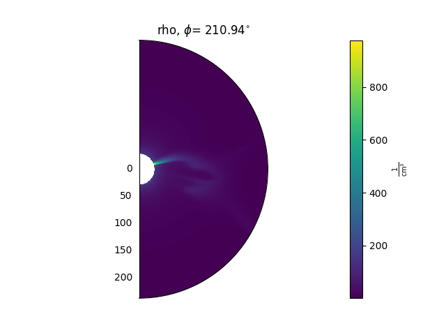
ax = plt.subplot(1, 1, 1, projection='polar')
model['rho'].plot_phi_cut(index, ax=ax, ...)
and produces an output like this:
For more examples of how to use these methods, see the Examples gallery.
Animating timesteps
If multiple timesteps have been loaded, each of the above methods can either be used to plot animations over time, or single time slices. By default they will produce animations which then need to be manually saved. As an example, to create and save an animated cut in the phi direction:
animation = model['rho'].plot_phi_cut(phi_index, ...)
animation.save('my_animation.mp4')
Contouring data
There are also methods that can be used to plot contours of the data on top of 2D slices. As an example, this can be helpful for plotting the heliospheric current sheet, by contouring \(B_{r} = 0\). These methods are
A typical use looks like this:
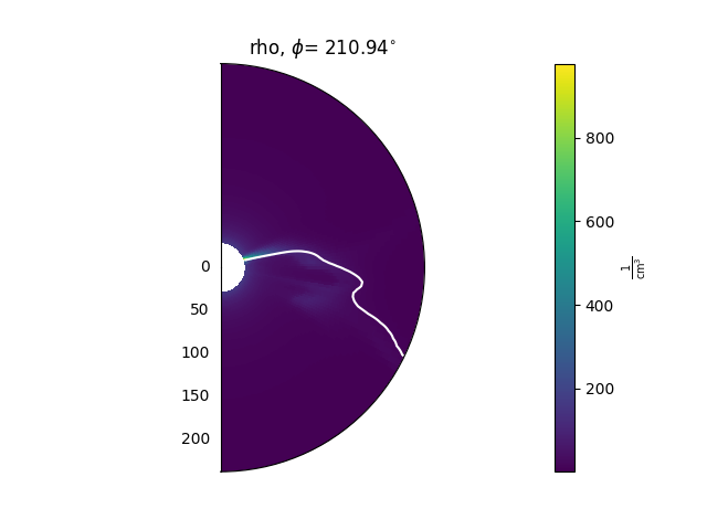
ax = plt.subplot(1, 1, 1, projection='polar')
model['rho'].plot_phi_cut(index, ax=ax, ...)
model['br'].contour_phi_cut(index, levels=[0], ax=ax, ...)
and produces outputs like this:
For more examples of how to use these methods, see the Examples gallery.
Normalising data before plotting
Sometimes it is helpful to multiply data by an expected radial falloff, e.g.
multiplying the density by \(r^{2}\). This can be done using the
Variable.radial_normalized method, e.g.:
rho = mas_output['rho']
rho_r_squared = rho.radial_normalized(2)
rho_r_squared.plot_phi_cut(...)