Sampling data from a 3D model

In this example we’ll see how to sample a 3D model output at arbitrary points within the model domain.

First, load the required modules.

from psipy.model import MASOutput
from psipy.data import sample_data

import astropy.constants as const
import astropy.units as u

import matplotlib.pyplot as plt
import numpy as np

Load a set of MAS output files, and get the number density variable from the model run.

mas_path = sample_data.mas_helio()
model = MASOutput(mas_path)
rho = model['rho']

Out:

Files Downloaded:   0%|          | 0/3 [00:00<?, ?file/s]

rho002.hdf:   0%|          | 0.00/8.02M [00:00<?, ?B/s]


vr002.hdf:   0%|          | 0.00/7.96M [00:00<?, ?B/s]



br002.hdf:   0%|          | 0.00/7.94M [00:00<?, ?B/s]

rho002.hdf:   0%|          | 3.00/8.02M [00:00<94:47:14, 23.5B/s]

rho002.hdf:   0%|          | 20.8k/8.02M [00:00<01:20, 98.8kB/s]

rho002.hdf:   1%|1         | 105k/8.02M [00:00<00:19, 397kB/s]

rho002.hdf:   4%|3         | 300k/8.02M [00:00<00:08, 899kB/s]

rho002.hdf:   9%|8         | 714k/8.02M [00:00<00:03, 1.96MB/s]

rho002.hdf:  18%|#8        | 1.46M/8.02M [00:00<00:01, 3.67MB/s]

rho002.hdf:  30%|##9       | 2.38M/8.02M [00:00<00:01, 5.40MB/s]

rho002.hdf:  40%|###9      | 3.17M/8.02M [00:00<00:00, 5.88MB/s]

rho002.hdf:  47%|####6     | 3.77M/8.02M [00:01<00:02, 1.59MB/s]

rho002.hdf:  57%|#####7    | 4.59M/8.02M [00:02<00:01, 2.23MB/s]

rho002.hdf:  64%|######3   | 5.10M/8.02M [00:02<00:01, 1.51MB/s]

rho002.hdf:  68%|######8   | 5.49M/8.02M [00:02<00:01, 1.70MB/s]

rho002.hdf:  78%|#######8  | 6.29M/8.02M [00:02<00:00, 2.44MB/s]

rho002.hdf:  95%|#########5| 7.62M/8.02M [00:03<00:00, 3.97MB/s]


Files Downloaded:  33%|###3      | 1/3 [00:03<00:06,  3.19s/file]


vr002.hdf:   0%|          | 100/7.96M [00:03<68:49:20, 32.1B/s]


vr002.hdf:   0%|          | 9.94k/7.96M [00:03<30:31, 4.34kB/s]


vr002.hdf:   1%|          | 53.4k/7.96M [00:03<04:29, 29.3kB/s]


vr002.hdf:   3%|2         | 205k/7.96M [00:03<00:54, 141kB/s]



br002.hdf:   0%|          | 100/7.94M [00:03<77:18:02, 28.5B/s]


vr002.hdf:   8%|8         | 658k/7.96M [00:03<00:12, 568kB/s]



br002.hdf:   0%|          | 10.9k/7.94M [00:03<31:26, 4.20kB/s]


vr002.hdf:  18%|#7        | 1.40M/7.96M [00:03<00:04, 1.41MB/s]



br002.hdf:   1%|          | 52.9k/7.94M [00:03<05:05, 25.8kB/s]


vr002.hdf:  22%|##2       | 1.79M/7.96M [00:03<00:03, 1.64MB/s]



br002.hdf:   2%|2         | 161k/7.94M [00:03<01:19, 97.9kB/s]


vr002.hdf:  27%|##7       | 2.18M/7.96M [00:03<00:03, 1.91MB/s]



br002.hdf:   7%|6         | 523k/7.94M [00:03<00:18, 403kB/s]


vr002.hdf:  36%|###6      | 2.88M/7.96M [00:04<00:01, 2.85MB/s]



br002.hdf:  16%|#6        | 1.30M/7.94M [00:04<00:05, 1.21MB/s]


vr002.hdf:  44%|####3     | 3.50M/7.96M [00:04<00:01, 3.53MB/s]


vr002.hdf:  53%|#####2    | 4.21M/7.96M [00:04<00:00, 4.21MB/s]


vr002.hdf:  60%|#####9    | 4.75M/7.96M [00:04<00:00, 3.65MB/s]



br002.hdf:  21%|##        | 1.65M/7.94M [00:04<00:07, 830kB/s]


vr002.hdf:  65%|######5   | 5.20M/7.96M [00:04<00:01, 2.41MB/s]



br002.hdf:  24%|##3       | 1.90M/7.94M [00:04<00:06, 968kB/s]


vr002.hdf:  74%|#######3  | 5.85M/7.96M [00:04<00:00, 3.04MB/s]



br002.hdf:  28%|##8       | 2.25M/7.94M [00:05<00:04, 1.25MB/s]


vr002.hdf:  82%|########1 | 6.49M/7.96M [00:05<00:00, 3.39MB/s]



br002.hdf:  41%|####1     | 3.27M/7.94M [00:05<00:01, 2.51MB/s]



br002.hdf:  54%|#####4    | 4.31M/7.94M [00:05<00:00, 3.85MB/s]



br002.hdf:  67%|######7   | 5.36M/7.94M [00:05<00:00, 5.13MB/s]


vr002.hdf:  87%|########7 | 6.92M/7.96M [00:05<00:00, 2.53MB/s]



br002.hdf:  81%|########1 | 6.47M/7.94M [00:05<00:00, 6.43MB/s]


vr002.hdf:  93%|#########3| 7.40M/7.96M [00:05<00:00, 2.69MB/s]



br002.hdf:  93%|#########2| 7.35M/7.94M [00:05<00:00, 6.96MB/s]



Files Downloaded:  67%|######6   | 2/3 [00:05<00:02,  2.82s/file]




Files Downloaded: 100%|##########| 3/3 [00:05<00:00,  1.92s/file]

Choose a set of 1D points to interpolate the model output at.

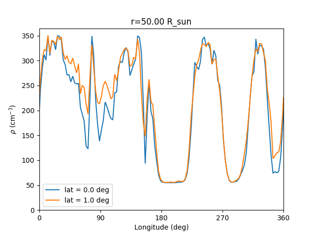
Here we keep a constant radius, and a set of longitudes that go all the way from 0 to 360 degrees. Then we choose two different, but close latitude values, and plot the results.

As expected, the values at 0 and 360 degrees are the same, and the profiles are similar, but different, due to the small difference in latitude.

fig, ax = plt.subplots()

npoints = 1000
r = 50 * np.ones(npoints) * const.R_sun
lon = np.linspace(0, 360, npoints) * u.deg

for latitude in [0, 1] * u.deg:
    lat = latitude * np.ones(npoints)
    samples = rho.sample_at_coords(lon, lat, r)

    ax.plot(lon, samples, label='lat = ' + str(latitude))

ax.legend()
ax.set_xlim(0, 360)
ax.set_ylim(bottom=0)
ax.set_xlabel('Longitude (deg)')
ax.set_ylabel(r'$\rho$ (cm$^{-3}$)')
ax.set_xticks([0, 90, 180, 270, 360])
plt.show()