Sampling data across timesteps

In this example we’ll see how to sample a 3D model across multiple timesteps.

First, load the required modules.

import astropy.units as u
import matplotlib.pyplot as plt
import numpy as np

from psipy.data import sample_data
from psipy.model import MASOutput

Load a set of MAS output files, and get the radial velocity variable from the model run. Note that there are multiple timesteps in the Variable object.

mas_path = sample_data.mas_helio_timesteps()
model = MASOutput(mas_path)
vr = model["vr"]
print(f"Number of timesteps: {vr.n_timesteps}")

  0%|                                              | 0.00/7.96M [00:00<?, ?B/s]
  1%|▍                                     | 98.3k/7.96M [00:00<00:10, 731kB/s]
  6%|██                                    | 442k/7.96M [00:00<00:04, 1.77MB/s]
 20%|███████▎                             | 1.57M/7.96M [00:00<00:01, 5.38MB/s]
 42%|███████████████▌                     | 3.34M/7.96M [00:00<00:00, 7.63MB/s]
 73%|██████████████████████████▉          | 5.79M/7.96M [00:00<00:00, 12.4MB/s]
 90%|█████████████████████████████████▎   | 7.17M/7.96M [00:00<00:00, 10.8MB/s]
  0%|                                              | 0.00/7.96M [00:00<?, ?B/s]
100%|█████████████████████████████████████| 7.96M/7.96M [00:00<00:00, 11.1GB/s]

  0%|                                              | 0.00/7.96M [00:00<?, ?B/s]
  1%|▍                                     | 98.3k/7.96M [00:00<00:10, 723kB/s]
  6%|██                                    | 442k/7.96M [00:00<00:04, 1.77MB/s]
 21%|███████▉                             | 1.70M/7.96M [00:00<00:01, 5.86MB/s]
 38%|██████████████                       | 3.01M/7.96M [00:00<00:00, 8.29MB/s]
 61%|██████████████████████▋              | 4.88M/7.96M [00:00<00:00, 11.7MB/s]
 87%|████████████████████████████████▎    | 6.96M/7.96M [00:00<00:00, 14.4MB/s]
  0%|                                              | 0.00/7.96M [00:00<?, ?B/s]
100%|█████████████████████████████████████| 7.96M/7.96M [00:00<00:00, 11.0GB/s]
Number of timesteps: 2

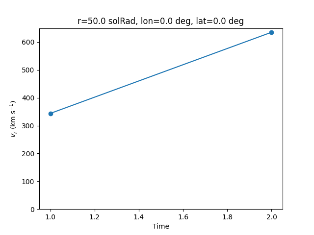
To sample across times, we’ll keep a constant spatial coordinate (r, lat, lon), but sample at each of the time coordiantes. This isn’t that exciting because there’s only two timesteps, but illustrates how it works!

fig, ax = plt.subplots()

t = vr.time_coords
r = 50 * u.R_sun * np.ones(len(t))
lon = 0 * u.deg * np.ones(len(t))
lat = 0 * u.deg * np.ones(len(t))

samples = vr.sample_at_coords(lon, lat, r, t)

ax.plot(t, samples, marker="o")

ax.set_ylim(bottom=0)
ax.set_xlabel("Time")
ax.set_ylabel(r"$v_{r}$ (km s$^{-1}$)")
ax.set_title(f"r={r[0]}, lon={lon[0]}, lat={lat[0]}")
plt.show()